I took a read at Ho's paper on denoising probabilistic diffusion models. It's a pretty dense paper, with an 3 paragraph introduction that probably could have been closer to 3 pages with the amount of details that it left out. This post is meant to be those 3 pages.

VAE's and ELBO Summarized

In generative models, we wish to estimate a data distribution $p_{\theta}(x)$. It is difficult in practice to force a single-function to capture everything about the data like:

• multi-modality
• long-range dependencies
• complicated geometry

To make modelling easier, we instead introduce latent variables $z$, so that we can write:

$$p_{\theta}(x) = \int p_{\theta}(x | z)p(z) \text{ dz}$$

This is a continuous mixture model, and representing $p_{\theta}(x)$ allows us to express complicated distributions while keeping $p_{\theta}(x | z)$ relatively simple. Of course in practice, $p_{\theta}(x | z)$ is also complicated (represented by a neural network).

Note that in general, evaluating this integral is intractable, because of the high-dimensional nature of $z$. This becomes problematic when trying to do inference (computing $p(z | x)$). Even though we can write $p(z | x) = \frac{p_{\theta}(x | z)p(z)}{p_{\theta}(x)}$, computing the denominator is intractable. Fortunately, introducing an approximate posterior distribution $q_{\phi}(z | x)$ allows us to give a lower-bound on the log-likelihood, as well as provide us a way to do inference.

Deriving the ELBO

We can write $\text{log }p_{\theta}(x)$ as follows:

$$\text{log }p_{\theta}(x)$$ $$= \text{log }\int p_{\theta}(x, z) \text{ dz}$$ $$= \text{log }\int p_{\theta}(x, z) \cdot \frac{q_{\phi}(z | x)}{q_{\phi}(z | x)}\text{ dz}$$ $$= \text{log }\mathbb{E}_{z \sim q_{\phi}(\cdot | x)}\left[ \frac{p_{\theta}(x, z)}{q_{\phi}(z | x)} \right]$$ $$\geq \mathbb{E}_{z \sim q_{\phi}(\cdot | x)}\left[ \text{log }\frac{p_{\theta}(x, z)}{q_{\phi}(z | x)} \right]$$

The last line is due to Jensen's inequality, and the quantity $\mathbb{E}_{z \sim q_{\phi}(\cdot | x)}\left[ \text{log }\frac{p_{\theta}(x, z)}{q_{\phi}(z | x)} \right]$ is known as the evidence-based lower bound (ELBO for short).

We can also rewrite the ELBO as follows:

$$\mathbb{E}_{z \sim q_{\phi}(\cdot | x)}\left[ \text{log }p_{\theta}(x) + \text{log }p_{\theta}(z | x) - \text{log }q_{\phi}(z | x) \right]$$

Rearranging, we get that:

$$\text{log }p_{\theta}(x) = \text{ELBO } + D_{KL}(q_{\phi}(z | x) \lVert p_{\theta}(z | x))$$

So the closer our estimated posterior $q_{\phi}$ matches the true posterior, the smaller the gap between the true log-likelihood and the ELBO lower-bound.

From our discussion so far, we face three core decisions:

• Defining and modelling the distribution of our latents $p(z)$
• Modelling the true posterior distribution $p_{\theta}(z | x)$
• Modelling the estimated posterior distribution $q_{\phi}(z | x)$

All about Multivariate Gaussians

Since all the core modelling choices are centered around Gaussians, it's helpful to review some properties about them. They will come in handy when we derive the training algorithms outlined in the DDPM paper.

Three Equivalent Definitions

There are three equivalent definitions of a multivariate gaussian:

A random variable $X = (X_1, X_2, \ldots, X_k)$ is a multivariate normal iff

1. There exist $\mu \in \mathbb{R}^k, A \in \mathbb{R}^{k \times l}$ such that $X = AZ + \mu$ where $Z = (Z_1, \ldots, Z_l)$ such that $Z_i \sim \mathcal{N}(0, 1)$ for all $1 \leq i \leq n$.
2. Every linear combination $Y = \sum_{i = 1}^k a_iX_i$ is normally distributed.
3. There exist $\mu \in \mathbb{R}^k$ and PSD matrix $\Sigma \in \mathbb{R}^{k \times k}$ such that $\phi_X(u) = \mathbb{E}\left[\text{exp}\left(iu^T\mu - \frac{1}{2}u^T\Sigma u\right)\right]$.

To prove equivalnce, we will prove that $1 \implies 2$, $2 \implies 3$, and $3 \implies 1$.

$1 \implies 2$:

We expand $Y = a^TX = a^T(AZ + \mu) = \sum{i = 1}^n (a^TA_i)Z_i + a^T\mu$ where $A_i$ is the $i$-th column of A. Since the $Z_i$'s are independent standard normal, we can conclude that $Y$ is also normally distributed with mean $\alpha^T\mu$ and variance $\sum{i = 1}^n (a^TA_i) = a^TAA^Ta$.

$2 \implies 3$:

Let $Y = u^TX$. From (2), we know that $Y$ is a normal distribution. Let $\mu(u), \sigma^2(u)$ denote the mean and variance of $Y$ (implicitly dependent on $\mu$). We can relate the characteristic functions of $X$ and $Y$ as follows:

$$\phi_X(u) = \mathbb{E}\left[\text{exp}\left(iu^TX\right)\right]$$ $$= \mathbb{E}\left[\text{exp}\left(iY\right)\right]$$ $$= \phi_Y(1)$$ $$= \text{exp}\left(i\mu(u) - \frac{1}{2}\sigma^2(u)\right)$$

We need to analyze the mean and variance of $Y$. It remains to show that $\mu(u) = u^T\mu$ and $\sigma^2(u) = u^T\Sigma u$ for some $\mu \in \mathbb{R}^k$ and PSD matrix $\Sigma \in \mathbb{R}^{k \times k}$. Define $\mu = (\mu_1, \ldots, \mu_k)$ where $\mu_i = \mathbb{E}[e_i^TX] = \mathbb{E}[X_i]$. We then have that $\mathbb{E}[Y] = \mathbb{E}[u^TX] = \sum_{i = 1}^k u_i\mathbb{E}[e_i^TX] = u^T\mu$.

We see that $\text{Var}(u^TX) = \sum_{i, j}u_iu_j\text{Cov}(X_i, X_j)$. Define $\Sigma \in \mathbb{R}^{k \times k}$ where $\Sigma_{ij} = \text{Cov}(X_i, X_j)$. Since $\Sigma$ is a covariance matrix, it is positive symmetric definite matrix by construction. Noting that $\sum_{i, j}u_iu_j\text{Cov}(X_i, X_j) = u^T\Sigma u$, we are done.

$3 \implies 1$:

Let $X$ be a random vector with characteristic function: $\phi_X(u) = \mathbb{E}\left[\text{exp}\left(iu^T\mu - \frac{1}{2}u^T\Sigma u\right)\right]$ for some $\mu \in \mathbb{R}^k$ and PSD matrix $\Sigma \in \mathbb{R}^{k \times k}$.

Since $\Sigma$ is a PSD matrix, it can be factored as $\Sigma = AA^T$. Define $Y = AZ + \mu$, where $Z = (Z_1, \ldots, Z_l)$ such that $Z_i \sim \mathcal{N}(0, 1)$ for all $1 \leq i \leq n$. We will show that the characteristic function of $Y$ is equal to that of $X$, completing the proof.

We have:

$$\phi_Y(u) = \mathbb{E}\left[\text{exp}\left(iu^TY\right)\right]$$ $$= \text{exp}\left(iu^T\mu\right) \cdot \mathbb{E}\left[\text{exp}\left(i(u^TA)Z\right)\right]$$

Let $b = A^Tu$. We can rewrite

$$\mathbb{E}\left[\text{exp}\left(i(u^TA)Z\right)\right] = \mathbb{E}\left[\text{exp}\left(ib^TZ\right)\right]$$

Since the $Z_i$'s are iid standard normals, $b^TZ \sim \mathcal{N}(0, b^Tb)$. Therefore,

$$\mathbb{E}\left[\text{exp}\left(ib^TZ\right)\right] = \text{exp}\left(-\frac{1}{2}b^Tb\right)$$ $$= \text{exp}\left(-\frac{1}{2}u^TAA^Tu\right)$$

We now have:

$$\phi_Y(u) = \text{exp}\left(iu^T\mu\right) \cdot \text{exp}\left(-\frac{1}{2}u^TAA^Tu\right)$$ $$= \text{exp}\left(iu^T\mu - \frac{1}{2}u^T\Sigma u\right)$$

as desired.

KL Divergence between of Multivariate Gaussians

We now state the formula for the KL divergence of two Gaussian variables. Given $p_1 \sim \mathcal{N}(\mu_1, \Sigma_1)$, $p_2 \sim \mathcal{N}(\mu_2, \Sigma_2)$, the KL divergence between the two distributions is:

$$\frac{1}{2} \left[\text{log}\frac{|\Sigma_2|}{|\Sigma_1|} - k + \text{Tr}\left(\Sigma_2^{-1}\Sigma\right) + (\mu_1 - \mu_2)^T\Sigma_2^{-1}(\mu_1 - \mu_2) \right]$$

To show this, start off with the fact that:

$$\text{log}p_1(x) = -\frac{k}{2} \text{log }2\pi - \frac{1}{2}\text{log}|\Sigma_1| - \frac{1}{2}(x - \mu_1)^T\Sigma_1^{-1}(x - \mu_1)$$

and

$$\text{log}p_2(x) = -\frac{k}{2} \text{log }2\pi - \frac{1}{2}\text{log}|\Sigma_2| - \frac{1}{2}(x - \mu_2)^T\Sigma_2^{-1}(x - \mu_2)$$

Therefore

$$\text{log}\frac{p_1(x)}{p_2(x)} = - \frac{1}{2}\text{log}\frac{|\Sigma_1|}{|\Sigma_2|} - \frac{1}{2}(x - \mu_1)^T\Sigma_1^{-1}(x - \mu_1) + \frac{1}{2}(x - \mu_2)^T\Sigma_2^{-1}(x - \mu_2)$$

From the definition of the KL divergence, we now proceed to take expectations under the distribution $p_1$. The first term is constant with respect to $x$. For the second term, we have that:

$$\mathbb{E}_{p_1}\left[-\frac{1}{2}(x - \mu_1)^T\Sigma_1^{-1}(x - \mu_1)\right] = -\frac{1}{2}\mathbb{E}_{p_1}\left[\text{Tr}\left((x - \mu_1)^T\Sigma_1^{-1}(x - \mu_1)\right)\right]$$ $$= -\frac{1}{2}\mathbb{E}_{p_1}\left[\text{Tr}\left(\Sigma_1^{-1}(x - \mu_1)(x - \mu_1)^T\right)\right]$$ $$= -\frac{1}{2}\text{Tr}\left(\Sigma_1^{-1}\mathbb{E}_{p_1}\left[(x - \mu_1)(x - \mu_1)^T\right]\right)$$ $$= -\frac{1}{2}\text{Tr}\left(\Sigma_1^{-1}\Sigma_1\right)$$ $$= -\frac{k}{2}$$

Now, onto calculating the third term. We introduce variables $y = x - \mu_1$ and $\delta = \mu_1 - \mu_2$. We can therefore rewrite

$$\mathbb{E}_{p_1}\left[\frac{1}{2}(x - \mu_2)^T\Sigma_2^{-1}(x - \mu_2)\right] = \mathbb{E}_{p_1}\left[\frac{1}{2}(y + \delta)^T\Sigma_2^{-1}(y + \delta)\right]$$ $$= \frac{1}{2}\mathbb{E}_{p_1}\left[y^T\Sigma_2^{-1}y + 2y^T\Sigma_2^{-1}\delta + \delta^T\delta\right]$$

The first term is $(X - \mu_1)^T\Sigma_2^{-1}(X - \mu_1)$, so taking expectations will give $\text{Tr}(\Sigma_2^{-1}\Sigma_1)$. Since $Y$ has zero mean, the expected value of the second term is 0. Finally the third term is constant, with value $(\mu_1 - \mu_2)^T\Sigma_2^{-1}(\mu_1 - \mu_2)$.

Putting this all together, we have the desired formula. Note for isotropic Gaussians of the form $\mathcal{N}(\mu, \beta I)$, the KL divergence simplifies to:

$$= \frac{1}{2\beta_2}\lVert\mu_1 - \mu_2\rVert_2^2 + C$$

where $C$ are some constant terms.

Denoising Probabilistic Diffusion Models

Let's go back to our modelling paradigm. Recall that we need to make three decisions:

• Defining and modelling the distribution of our latents $p(z)$
• Modelling the true posterior distribution $p_{\theta}(z | x)$
• Modelling the estimated posterior distribution $q_{\phi}(z | x)$

In the DDPM paper, they make the following choices:

• $z$ is a sequence of latent variables obtained by an iterative denoising process. In particular, they start out with a data point $x_T \sim \mathcal{N}(0, I)$, and model the sequence $x_{T - 1}, \ldots, x_1$ via a Markov chain with Gaussain transitions. Note that $x_0 \sim q(x_0)$ is the actual data.
• the true posterior distribution is an iterative denoising process where $x_{t - 1} = \mathcal{N}(\mu(x_t, t), \Sigma(x_t, t))$ where $\mu_{\theta}(\cdot), \Sigma_{\theta}(\cdot)$ are learned functions.
• the approximate distribution $q(x_{1:T} | x_0)$ is also fixed to a markov chain witht the following transition rule: $x_t = \mathcal{N}(x_{t - 1}, \beta_t I)$ where $1 \leq t \leq T$ and $\beta_t$ is a predefined variance schedule. This process is called the forward process or the diffusion process.

ELBO for Diffusion Models

For training, we wish to minimize the log-likelihood of the data, or to maximize the negative ELBO as a proxy. We write the ELBO as follows:

$$\mathbb{E}_q\left[-\text{log}\frac{p_{\theta}(x_{0:T})}{q(x_{1:T} | x_0)}\right] = \mathbb{E}_q\left[ -\text{log}p_{\theta}(x_T) - \sum_{t \geq 1}\text{log}\frac{p_{\theta}(x_{t-1}|x_t)}{q(x_t | x_{t - 1})} \right]$$

We can further rewrite this as:

$$\mathbb{E}_q\left[ D_{KL}(q(x_T | x_0) \lVert p_{\theta}(x_T)) + \sum_{t > 1} D_{KL}(q(x_{t - 1} | x_t, x_0) \lVert p_{\theta}(x_{t - 1} | x_t)) - \text{log } p_{\theta}(x_0 | x_1) \right]$$

Deriving the Simplified Loss Function for Training

In the DDPM paper, they ignore the first and last terms of the loss function and focus solely on optimizing the $D_{KL}(q(x_{t - 1} | x_t, x_0) \lVert p_{\theta}(x_{t - 1} | x_t))$ terms. A nice fact is that $q(x_{t - 1} | x_t, x_0)$ is gaussian with mean $\tilde{\mu_t}(x_t, x_0)$ and covariance $\tilde{\beta_t}I$ where

$$\tilde{\mu_t}(x_t, x_0) = \frac{\sqrt{\overline{\alpha_{t - 1}}}\beta_t}{1 - \overline{\alpha_t}}x_0 + \frac{\sqrt{\alpha_t (1 - \overline{\alpha_{t - 1}})}}{1 - \overline{\alpha_t}}x_t$$

and

$$\tilde{\beta_t} = \frac{1 - \overline{\alpha_{t - 1}}}{1 - \overline{\alpha_t}}\beta_t$$

In the paper, they make the simplification that $\Sigma_{\theta}(x_t, t) = \sigma_t^2I$ where $\sigma_t^2$ set to either $\beta_t$ or $\overline{\beta_t}$. Since each KL term in the loss is between two gaussians, we can write each term (dropping constants) as:

$$\mathbb{E}_q\left[\frac{1}{2\sigma_t^2}\lVert \tilde{\mu_t}(x_t, x_0) - \mu_{\theta}(x_t, t) \rVert^2\right]$$

From the relation, $x_t = \sqrt{\overline{\alpha_t}}x_0 + \sqrt{1 - \overline{\alpha_t}}\epsilon$, we can write $x_0 = \frac{1}{\sqrt{\overline{\alpha_t}}}\left(x_t - \sqrt{1 - \overline{\alpha_t}}\epsilon\right)$ and substitute:

$$\mathbb{E}_{x_0, \epsilon}\left[ \frac{1}{2\sigma_t^2}\lVert \frac{1}{\sqrt{\alpha_t}}\left( x_t - \frac{\beta_t}{\sqrt{1 - \overline{\alpha_t}}} \right) - \mu_{\theta}(x_t, t) \rVert^2 \right]$$

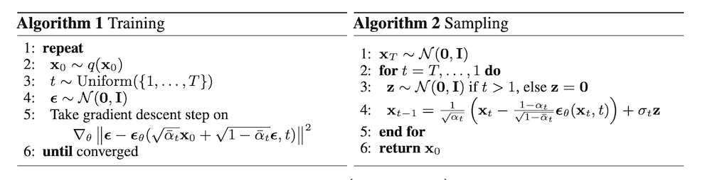
What we have here is a regression problem where the learned mean $\mu_{\theta}$ needs to predict $\frac{1}{\sqrt{\alpha_t}}\left(x_t - \frac{\beta_t}{\sqrt{1 - \overline{\alpha_t}}}\epsilon\right)$. Instead of predicting the mean directly, we predict the noise given a timestep $t$ and $x_t$. From this, we know that the estimated $x_0$ is $\frac{1}{\sqrt{\overline{\alpha_t}}}\left(x_t - \sqrt{1 - \overline{\alpha_t}}\epsilon_{\theta}(x_t, t)\right)$, where $\epsilon_{\theta}$ is our learned model. Plugging this into the formula for $\tilde{\mu}$, we have that

$$\mu_{\theta}(x_t, t) = \frac{1}{\sqrt{\alpha_t}}\left(x_t - \frac{\beta_t}{\sqrt{1 - \overline{\alpha_t}}}\epsilon_{\theta}(x_t, t) \right)$$

During sampling we iteratively apply the rule $x_t = \mu_{\theta}(x_t, t) + \sigma_t^2 z$ where $z$ is a standard Gaussian.

Using the reparameterized noise model, we have that:

$$\mathbb{E}_q\left[\frac{1}{2\sigma_t^2}\lVert \tilde{\mu_t}(x_t, x_0) - \mu_{\theta}(x_t, t) \rVert^2\right] = \mathbb{E}_{x_0, \epsilon}\left[ \frac{\beta_t^2}{2\sigma_t^2\alpha_t(1 - \overline{\alpha_t})} \lVert \epsilon - \epsilon_{\theta}(x_t, t)\rVert^2 \right]$$

The DDPM paper drops the constant in front of the squared-norm.

Here is the pseudocode for training and sampling.